(Image by James Vaughan)
If you’ve ever tried to set up a legitimate statistical test in Excel, you already know it’s painful, but if you have the Analysis ToolPak enabled, things get a bit easier. Today, we’re going to learn how to run statistical tests in Excel. We’ll cover F-tests to compare variances, t-tests to compare 2 averages, and ANOVAs to compare multiple averages.
A word of warning: the ToolPak might seem self explanatory, but some of the results are easy to interpret incorrectly.
This post should take between 22 and 44 minutes to read and toy with. Alright, let’s go ahead and get started.
Compare Variances With an F-Test
Before you compare two sample averages, it’s usually a good idea to to compare their variances first. We do this using an F-test. This can also be a good way to compare 2 treatments in order to see if one of them produces more consistent results.
WARNING: F-tests assume that your sample data comes from a normal distribution. Worse, Excel offers zero normality testing capabilities. To be genuinely rigorous, you would need to build your own normality test. (Or, you could download this normality test excel spreadsheet I put together for you.)
With that caveat out of the way, let’s say you wanted to compare two samples, each of them made up of units that you randomly assigned to one of two treatments, like this:
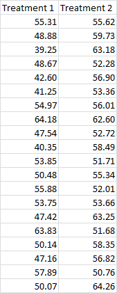
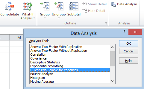
Start off by clicking the Data tab, then head over to the Analysis section, and hit Data Analysis. Now select F-Test Two-Sample for Variances and hit OK.
You’ll get this screen:
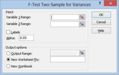
Now click in the Variable 1 Range box and select your first treatment data:
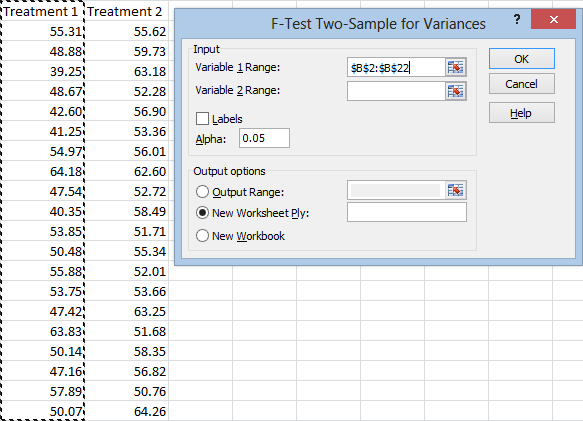
And do the same for the second treatment. Notice that I’m selecting the headers as well as the data. Click the Labels box so that Excel can use these headers properly.
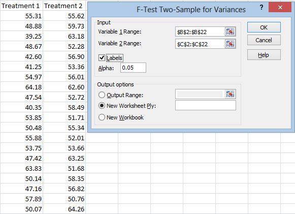
Your Alpha is your level of statistical significance. An alpha of 0.05 means that we can be 95 percent confident in our solution. (To be more precise, it means that if there is no true difference between the variances, 5 percent of the time we will falsely conclude that there is a difference.)
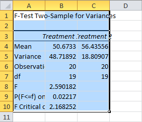
Under Output options, you can choose Output Range and select where to paste your data. You can also choose to set up a New Workbook and save the results to a new file. I’ll just leave it on New Worksheet Ply. The results will be posted in a new worksheet on the same project. Now just hit OK. Let’s take a look at the results:
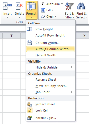
To “prettify” this, click the Home tab, head over to the Cells section, click Format, and hit AutoFit Column Width:
Now let’s take a look at what this all means:
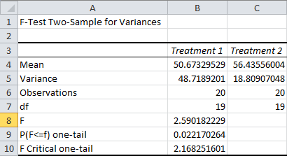
The Means and Variances should be self-explanatory. (As a quick reminder, the variance is the average squared distance of your sample points from the mean. It’s the standard deviation squared.) Observations is the sample size, and df represents your degrees of freedom derived from the sample size.
F is your computed F-Statistic. It’s a ratio of the two variances. The F Critical one-tail is the cutoff point for the Alpha we chose, of 5%. In other words, if the F-Statistic were smaller than 2.17, we couldn’t claim with 95 percent confidence that the variances were different.
This in itself is useful information. At this sample size, one of the sample variances needs to be over twice as large as the other for us to detect a significant difference. This can be a quick and easy way to evaluate the statistical power of this test before you set it up. With power this weak, it might be worth assuming your variances are different, even if the results are inconclusive.
The P(F<=f) one-tail is the one-tailed p-value for our F-test.
Warning: Excel’s p-value is based on a one-tailed test. This is usually the right choice for an F-test, but it’s dead wrong here. The reason for this is there are actually two ways for the variances to be different. Either the first variance is larger, or the second variance is larger.
You need to double this p-value to get the correct result.
In this case, the results are still conclusive. Our p-value is 4.4%, which is below our cutoff Alpha of 5%. (This means that if the true variances are identical, there is only a 4.4% chance that the sample variances would be at least this different.)
Unlike some statistical packages, Excel doesn’t reorganize the data so that the larger variance is always the numerator for the test. Here’s what would have happened if we ran the test with the treatments reversed:
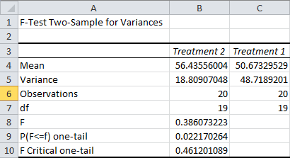
In this case, an F-statistic smaller than the F Critical one-tail is what we need in order to conclude that the variances are different. This is how you should approach things if your F-statistic is less than 1.
In either case, if you double your p-value and it’s less than your alpha, you know you have significantly different variances.
Compare Averages With a t-Test
Once you’ve tested the variances, you can go ahead and compare the averages between the two samples. This will let you know whether the treatment had a statistically significant impact on the results.
(The t-tests are typically safe if your sample size is over 15, even if they don’t come from a normal distribution, as long as there’s no strong skewness. If the sample size is over 40, you don’t even need to worry about that.)
There are three ways you can compare the samples: a t-test assuming equal variances, a t-test assuming unequal variances, and a paired t-test.
If your F-test turned up unequal variances, like it did in the last example, you should obviously use the t-test assuming unequal variances.
But if your F-test didn’t reach significance, I wouldn’t necessarily dive right into the assumption of equal variance.
As I pointed out in the previous example, one of your sample variances would need to be twice as large as the other (with that sample size) in order to say the difference was statistically significant. Your F-test isn’t going to have a lot of statistical power in many cases. Unless your sample size is large enough to keep the range for this difference small, I’d still recommend assuming unequal variances.
If you feel confident that the difference between your variances is very small or nonexistent, a t-test that assumes equal variances can give more accurate results, but assuming unequal variances is always the more conservative option.
The paired t-test is based on a different experimental setup. Use this if, instead of randomly assigning half of your units to one treatment and half of them to the other, you assign all of your units to both treatments. Ideally, you would randomly assign half of the units to receive the first treatment before the second, and the other half to receive the second treatment before the first.
No matter which t-test you use, the process in Excel is pretty much identical, so make sure you choose the correct t-test.
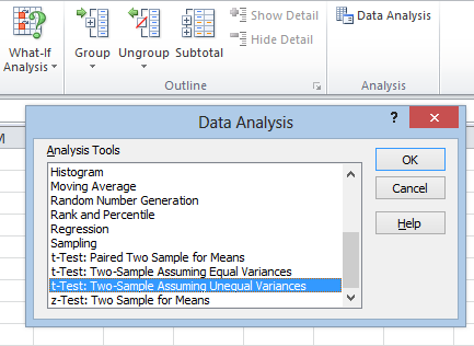
Start by hitting the Data tab, then head over to the Analysis section and hit Data Analysis. When the window pops up, choose the correct t-test based on my guidelines above, and then hit OK:
No matter which t-test you select, a window will pop up that looks almost exactly like this one (with the title of the window being the only difference):
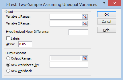
Now fill the Variable 1 Range and Variable 2 Range, making sure to check the Labels box if you include the title rows with your data:
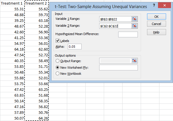 At this point, you can go ahead and hit OK if you like. However, I’d like to point out the Hypothesized Mean Difference box. Excel doesn’t have a whole lot of features that I prefer over more advanced statistical packages, but this box is nice to have. If you leave it alone, Excel will just test whether there’s a statistically significant difference between the averages of your 2 samples. But if you put a number in this box, Excel will test whether the difference is statistically different from a number you choose. This allows you to test a more elaborate prediction about how your treatments are influencing your results.
And, of course, under Output options, you can select whether to paste the output of the test onto the same sheet with the Output Range, a new sheet on the same workbook with New Worksheet Ply, or a new file with New Workbook.
Now let’s take a look at the results I get after hitting OK.
Here are the results I get from a t-test assuming unequal variances:
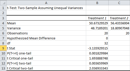
As before, the Mean and Variance rows are self-explanatory, the Observations row is your sample size for each sample, and df represents your degrees of freedom. The Hypothesized Mean Difference is the difference between the two samples that you are testing for. Remember that these tests can only “accept” a difference within a specific range, and it’s more appropriate to say that you “failed to reject” the hypothesis.
The t Stat row lists the t-statistic for your test. This measures the distance between your sample averages in standard deviations. In this case, Treatment 1′s average was 3.14 standard deviations below Treatment 2′s average.
The P(T<=t) one-tail is the one-tailed p-value for the test, and the t Critical one-tail is the one-tailed cutoff value for our t-statistic. The two-tailed equivalents are listed next.
So, do you use the one-tailed or the two-tailed results? It depends what you’re testing. If you were just testing whether the two treatments were different from each other, or trying to figure out which treatment was better, you should use the two-tailed test. But if you were testing whether a specific treatment were better, you should use the one-tailed test.
In this case, both tests reach significance. As a reminder, a p-value of 0.004, as in the two-tailed test, means that if the difference between our true averages were zero (or whatever we chose as our hypothesized difference), we would expect to get a t-statistic at least this high only 0.4% of the time.
Here are the results I get after running a t-test assuming equal variances:
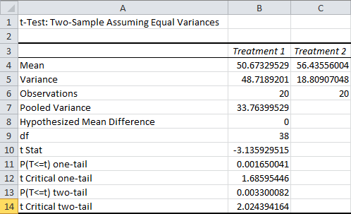
Most of the row labels are the same, but the values are different. The p-value, for example, is smaller. Like I said, this is a less rigorous test. (This is also one of many reasons why you should never just go off of the p-value without looking at the methods.)
The only new row here is the Pooled Variance, which is an estimate of the true variance, assuming that both samples share the same variance.
Finally, here are the results I get after running a paired t-test:
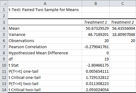
Remember, only use this test if you assigned all of your units to both treatments. Like I said, it’s best if half of your units are randomly assigned to take treatment 1 first, and half of your units are randomly assigned to take treatment 2 first.
The only new row you’ll see here is the Pearson Correlation. This is the correlation between the value on the first treatment, and the value on the second treatment. This tells you how much influence the value on the first treatment has over the value on the second treatment (or vice versa).
In addition to the t-tests, Excel offers a z-test. This is an idealized test that’s typically only useful for students learning how statistical tests work. It requires you to know the standard deviation of the entire population, something that you’ll almost never have access to. Z-tests have little or no practical application, so I’m skipping over it.
Instead, we’ll take a look at the ANOVA capabilities.
How to Run a One-Way ANOVA in Excel
While t-tests are a convenient way to compare two different treatments with each other, sometimes we need to compare more. To do this, we need to run a one-way ANOVA. (Like the F-test, ANOVAs assume your data comes from a normal distribution. This is something you would need to test, but unfortunately Excel doesn’t offer an easy way to pull that off.) For the sake of argument, let’s say you had to compare three different treatments with each other, like this:
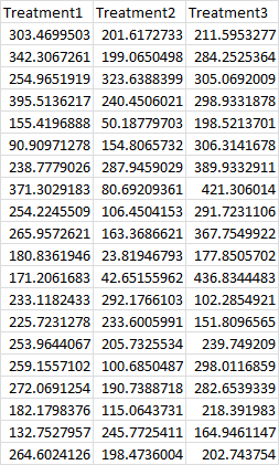
To compare them, we’d click the Data tab, head over to the Analysis section, and hit Data Analysis. Then we’d select Anova: Single Factor (for a one-way ANOVA), and hit OK:
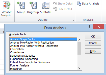
That will take us to this window:
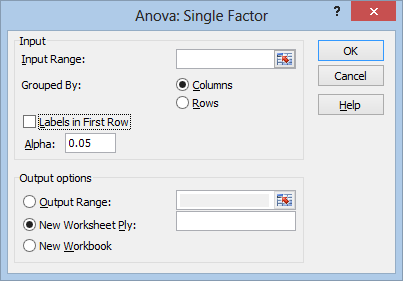
Now just click in the Input Range box and select your data. Make sure to check Labels in First Row if you select your data headings. As always, under Output options you can choose to paste the results in a specific place (Output Range), on a new sheet (New Worksheet Ply), or a new file (New Workbook).
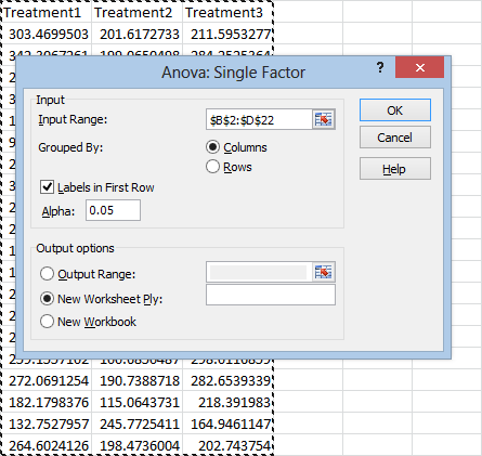
Now just hit OK. Your results will look something like this (after you fit the columns):
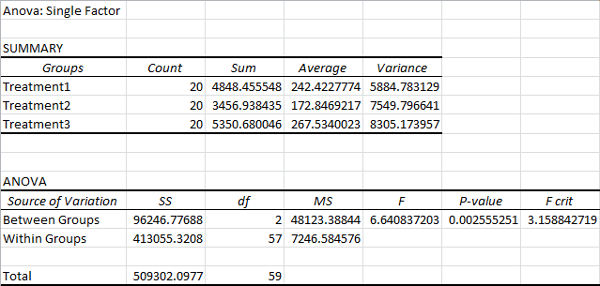
In the Summary section, you can compare the basic stats of the three treatments. The treatments are listed under the Groups column, followed by the Count, Sum, Average, and Variance columns. This should all be pretty self explanatory. (As a reminder, variance is the average squared distance of your samples from the mean. It’s the standard deviation squared.)
The ANOVA is your Analysis of Variance.
The Source of Variation column tells you which variance you’re looking at. Between Groups explores the variance that is explained by the treatments involved. Within Groups explores the variance within each treatment, which still has no explanation. The Total row explores the variance of all your samples. It’s just the sum of explained and unexplained variance.
The SS column displays the Sum of Squares for each row. This is a sum of the squared distance from the expected value.
df displays the degrees of freedom for each row.
(Here, there are 2 degrees of freedom for between group variation, since we can fully describe the variance between groups using 2 distances from any one of the 3 groups. There are 57 degrees of freedom for within group variation, since each group’s variation can be fully described as 19 distances from any one of the 20 points in that group. There are 59 degrees of freedom for the total variance, since the variation can be explained as 59 distances from any one of the 60 sample points.)
MS represents Mean Squared Error, which is just the sum of squares divided by the degrees of freedom. In other words, it’s the average squared distance from the expected value.
The F column lists your F-statistic. It’s a ratio of the between group mean squared error over the within group mean squared error. In other words, it’s a ratio of explained variance over unexplained variance.
The most important statistic is your P-value. If it’s below your cutoff value (typically 0.05), you can be pretty safe in assuming that at least one of your treatments produced different results from the others. That doesn’t mean all of your treatments are different. To find out which specific treatments are different from each other, you need to perform individual t-tests between them. (Technically, you would need to run a simultaneous test like a Tukey Multiple Comparison procedure, but Excel doesn’t offer a native solution for that. This is important, but it’s a subject for another day.)
(I know I keep stressing this, but as a reminder, the p-value operates on the assumption that your null hypothesis is true. Here, it means that if there is no real difference between the three treatments, there is only a 0.2 percent chance that our F-statistic would be at least this high. It does not mean that there is only a 0.2 percent chance that the null hypothesis is true. It’s impossible to reach conclusions like that using frequentist statistics. I talk more about p-values and statistical tests here.)
How to Run a Two-Way ANOVA in Excel
(If you only have one sample point for each variable combination, skip down to the section below on two-way ANOVAs without replication.)
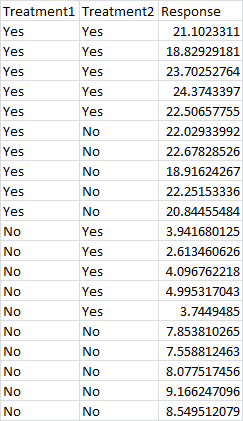
Sometimes it’s not enough to compare treatments with each other. Sometimes we need to see what happens when we combine two treatments with each other. In order to do that, we need to perform a two-way ANOVA, which Excel calls a Two-Factor ANOVA. So, if your mind works like mine, this is probably how you would expect to organize your data for this tool:
Unfortunately, for some reason, this isn’t what the Analysis ToolPak is looking for. Instead, it’s looking for something formatted in a much less less obvious way (to me). Here’s the format they’re looking for:
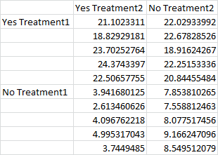
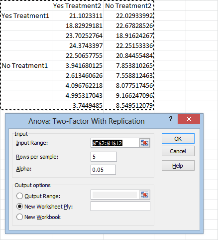
Here the data is divided into quadrants. The top left is yes-yes, the top right is yes-no, the bottom left is no-yes, and the bottom right is no-no. The data doesn’t actually need to be labeled “yes” and “no” like this, and these could be categorical variables with more than just yes/no values. (For example, the top row could read treatment 1, treatment 2, treatment 3, and the left column could read brand 1, brand 2, brand 3.) For each combination, you must have the same number of sample points. In this case, there are 5 samples for each combination.
As usual we get to the ToolPak by clicking the Data tab, heading over to the Analysis section, and hitting Data Analysis. Then just select Anova: Two-Factor With Replication and hit OK:
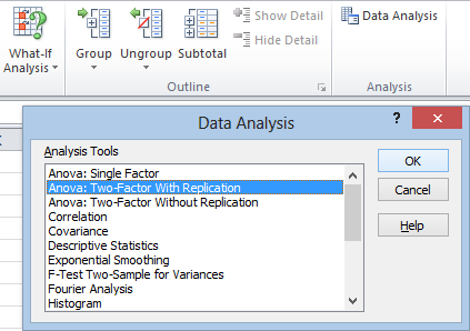
Here’s what the window looks like:
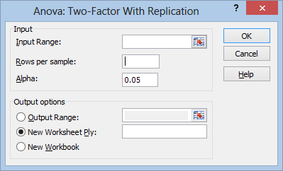
In the Rows per sample box, you’ll enter the number of replications for each treatment combination (in this case 5). Now just click in the Input Range box, select your data, choose where you want to output the result, and hit OK:
Your results will look something like this:
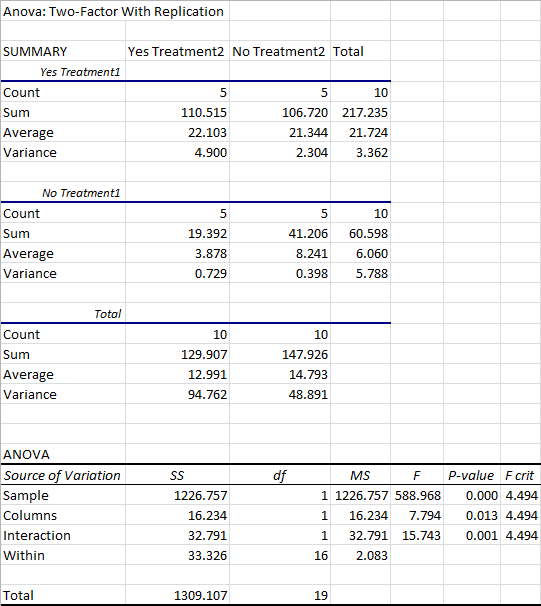
The results are split into two general sections: the Summary, which lists the count, sum, average, and variance for each combination of treatments, and the ANOVA at the bottom, which shows you the results of the test.
The Summary is pretty self-explanatory. You have a column for each treatment of one variable (in this case, yes or no for Treatment2), as well as a “Total” column that ignores this variable.
These results are then split into a separate section for each treatment of the other variable (in this case, yes or no for Treatment1). There’s also a section for the “Total” results, ignoring the influence of this variable.
The ANOVA is a little difficult to read, unfortunately, because it doesn’t use any of the labels you provided it. Let’s go over these.
Sample: This row analyzes the variance attributed to the the treatments listed in the 1st column, when you first set up the data. In this case, it’s analyzing the variance attributed to the presence or absence of Treatment1.
Columns: This row analyzes the variance attributed to the treatments listed in the 1st row. In this case, it’s referring to the presence or absence of Treatment2.
Interaction: This row analyzes the variance attributed to the interaction between both treatments. If this reaches significance, it means that the presence of both treatments will lead to results different from a simple sum of the effects explained by the treatments in isolation.
As always, the most important statistic here is the P-value. If it’s less than your cutoff value (usually 0.05), you will assume that the results are statistically significant.
From an ANOVA, it’s not immediately obvious exactly how the variables influence the outcome. In this example, while our p-values tell us that both variables are influencing the results, and that the interaction between those variables is influencing them as well, we can’t immediately tell which combination of treatments is best.
If bigger numbers were better results, for example, the summary data suggests we should use Treatment1 and Treatment2. But the ANOVA can’t tell us if this is actually superior to Treatment1 without Treatment2. The averages are still pretty close to each other, and the ANOVA doesn’t tell us whether the difference is statistically significant. We would want to compare these with a t-test before assuming that one option were better than the other.
Two-Way ANOVA Without Replication
Sometimes you only have one sample point for each combination, like this:

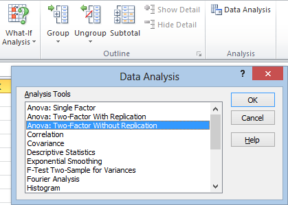
In this case, you’ll need to do a two-way ANOVA without replication:
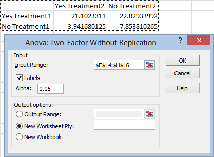
By now, you should be able to figure out what to do. Just click in the Input Range box and select your data. Make sure to check the Labels box if you select your headings.
The output will look something like this:
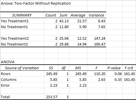
Most of this should be pretty self-explanatory. Again, the ANOVA isn’t labeled in a way that makes a whole lot of sense. Rows represents the variation explained by the variables listed in the your first column (in this case, yes or no for Treatment1). Columns represents the variation explained by the variables in the first row of your data (in this case, yes or no for Treatment2).
As you can see, our p-values failed to reach significance at the 0.05 level. This is pretty common for ANOVAs without replication.
Alright, that wraps up this session. The ToolPak doesn’t offer any other boilerplate statistical tests, so if you need to perform them, you’ll need to build them yourself. I might revisit that in the future.
Thanks for reading. Be sure to subscribe below if you want to see more updates like this one.
