One of the primary goals of statistical process control is to reduce the probability of a “defect,” however you define it, to acceptable levels.

Probably the most widely known example is Six Sigma, which aims to keep the number of defects below 3.4 per million. (More on that later, considering that it technically corresponds to 4.5 sigma.)

Defects are often measured in PPM (parts per million), but statistical processes are usually understood in terms of standard deviations (sigma).

The terminology DPMO (defects per million opportunities) is also sometimes used in place of PPM, but it means essentially the same thing.

It should go without saying that being able to convert back and forth between PPM and sigma can be very handy. I went ahead and put together a “calculator” for you to accomplish this (okay, it’s an Excel spreadsheet). You can use the calculator to convert between PPM and sigma in both traditional Statistical Process Control and Six Sigma (and yes, the results are different).

To get the calculator, and to sign up for more updates like this one, go ahead and sign up using the form below. (I will never share your email address with anybody.) Or you can go ahead and read on to understand how this conversion works, and set it up yourself.

The Direct Conversion Between PPM and Sigma (As In, Not the Six Sigma Conversion)

So, as is typical in engineering, we assume that our process errors are going to stick to the normal distribution. (That’s not always a safe assumption, by the way. If you sign up for the calculator, you’ll also get access to my other spreadsheets, a normality test included.)

Operating under that assumption, the direct conversion between PPM and Sigma is pretty straightforward. We use the standard normal distribution, with its mean of 0 and its standard deviation (sigma) of 1.

From Sigma to PPM

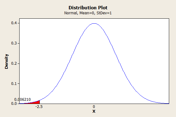
So, if we wanted to know the PPM that corresponded to 2.5 sigma, we could use -2.5 as our Z value and use it to find the probability, like so:

In Excel, you could find this using the formula =NORMSDIST(-2.5). (I’m giving away the secrets of my spreadsheet here.)

If you’re wondering about that negative sign, let me explain. Excel and most other calculators use the cumulative normal distribution to calculate values. That means they start from the left and work their way forward. If we entered =NORMSDIST(2.5), we would get 1-0.006210 as our answer. We could certainly work with that; it’s just not as convenient.

So, 0.006210 is a probability. To get this into PPM, we would multiply by a million.

That gives us 6209.665326 PPM. (No, 2.5 sigma isn’t very good.)

From PPM to Sigma

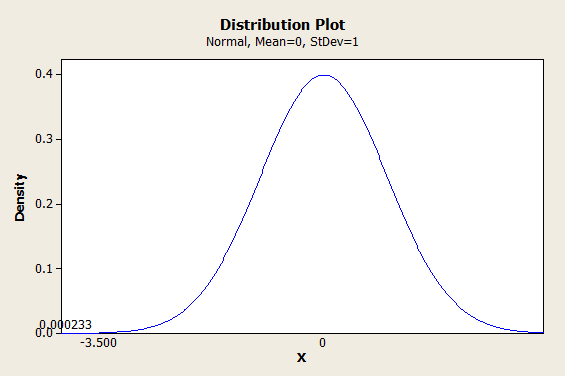
Alright, let’s say we wanted to go from 233 PPM to sigma. First, we need to get this from PPM to a probability. So we divide by a million and get 0.000233. Now, we input this probability into the inverse standard normal distribution and find our z-value (sigma), like so:

So 233 PPM corresponds to about 3.5 sigma. In Excel, we could find this using =-NORMSINV(0.000233), which gives us 3.499575281. (The negative sign in the formula counteracts the fact that we’re dealing with the left tail of the distribution.)

Conversion Between PPM and Sigma With the 1.5 Sigma Shift (As In, The Six Sigma Fanboys Can Pay Attention Now)

Okay, here’s where things get just a little bit more tricky (or as statistician Donald J. Wheeler has said dismissively, “goofy.”)

The Six Sigma method doesn’t use a straightforward measure of sigma. Instead, they implement a 1.5 sigma shift.

Now, if that sounds arbitrary, it sort of is (some even call it an abomination). However, there is an origin story behind the shift, and if you understand why it exists, there is a method to the madness.

The 1.5 sigma shift has it’s origins in the world of control charts. When Walter Shewhart developed his model for statistical quality control in the 1920s, he recommended using a series of small samples, rather than a single large sample. This reduces sampling costs, for obvious reasons.

In particular, he recommended taking sample sizes of 4, because it simplified calculations and personal computers were a long way off.

As we all know, in the real world, processes don’t run according to plan forever. Systems run off track. Your mean values are going to drift away from the ideal.

Here’s the punchline.

A sample size of 4 is capable of detecting a minimum shift in the mean of 1.5 sigma.

So, Six Sigma is (supposed to be) based on the assumption that your last sample (of size 4) could have been from a batch where your mean shifted as much as 1.5 sigma, and you weren’t able to detect it.

Unfortunately, it seems like very few people understand this bit of arcane knowledge, and this can lead to all kinds of confusion, including the misconception that 3.4 PPM actually corresponds to 6 standard deviations, when it really corresponds to 4.5.

A more rigorous approach, inspired by Six Sigma but with a little less dogma, would implement a shift of however many sigma your last sample could reasonably detect, rather than simply assuming 1.5, since sample sizes rarely stick to exactly 4.

Anyway…

From Sigma to PPM, With the 1.5 Sigma Shift

And now, a demonstration of why a Six Sigma process is said to keep your PPM below 3.4.

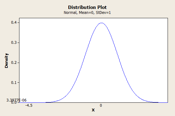
We start with 6 sigma, and we assume that our last sample (of size 4) was unable to detect a shift in the mean of 1.5 sigma. So we subtract 6-1.5=4.5. Then we use -4.5 as our Z-score and plug it into the cumulative normal distribution:

Ta da! We multiply 3.3977 * 10^-6 by a million and we get 3.3977 PPM, which is basically 3.4.

From PPM to Sigma, With the 1.5 Sigma Shift (Careful With This!)

Now here’s where the 1.5 sigma shift can start to look like a con if you aren’t careful. Try not to con yourself with it. I very rarely use exclamation points but seriously, be careful!

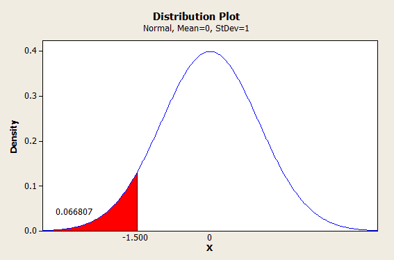
So let’s say our samples are telling us that our PPM is at 66,807, and we want to see that in sigma. Well, we’d start by dividing that by a million to get 0.066807 for our probability. Then we would plug that probability into the inverse standard normal distribution to get our Z-score (sigma):

(The number of defects is starting to look more like real life, isn’t it?)

So we find ourselves at 1.5 sigma. But hang on, don’t forget the 1.5 sigma shift. So now we add 1.5+1.5 = 3 sigma.

Neat?

Okay. Let me level with you. I’m not comfortable with saying that almost 7 percent of our products are defective, and that we’re going to just go ahead and call that 3 sigma. You shouldn’t be either, and that’s not how you should be using this conversion.

I would advise against ever using this conversion on data from an actual sample. Instead, I would recommend only using this conversion theoretically. 

For example, if you are guaranteeing to a customer that your DPMO is 233 or lower, then you could use this conversion in order to be conservative. The direct conversion from 233 PPM would be 3.5 sigma, but to be conservative, you would aim to put 5 sigma between your mean and your defect limits, not 3.5.

Get it?

Ready to download that PPM to sigma, sigma to PPM calculator? Go ahead and sign up for it, and similar updates, right here: